
1.4: An example of the variational theory: The \(H_2^+\) molecule ion
- Page ID
- 20868

\( \newcommand{\vecs}[1]{\overset { \scriptstyle \rightharpoonup} {\mathbf{#1}} } \)
\( \newcommand{\vecd}[1]{\overset{-\!-\!\rightharpoonup}{\vphantom{a}\smash {#1}}} \)
\( \newcommand{\id}{\mathrm{id}}\) \( \newcommand{\Span}{\mathrm{span}}\)
( \newcommand{\kernel}{\mathrm{null}\,}\) \( \newcommand{\range}{\mathrm{range}\,}\)
\( \newcommand{\RealPart}{\mathrm{Re}}\) \( \newcommand{\ImaginaryPart}{\mathrm{Im}}\)
\( \newcommand{\Argument}{\mathrm{Arg}}\) \( \newcommand{\norm}[1]{\| #1 \|}\)
\( \newcommand{\inner}[2]{\langle #1, #2 \rangle}\)
\( \newcommand{\Span}{\mathrm{span}}\)
\( \newcommand{\id}{\mathrm{id}}\)
\( \newcommand{\Span}{\mathrm{span}}\)
\( \newcommand{\kernel}{\mathrm{null}\,}\)
\( \newcommand{\range}{\mathrm{range}\,}\)
\( \newcommand{\RealPart}{\mathrm{Re}}\)
\( \newcommand{\ImaginaryPart}{\mathrm{Im}}\)
\( \newcommand{\Argument}{\mathrm{Arg}}\)
\( \newcommand{\norm}[1]{\| #1 \|}\)
\( \newcommand{\inner}[2]{\langle #1, #2 \rangle}\)
\( \newcommand{\Span}{\mathrm{span}}\) \( \newcommand{\AA}{\unicode[.8,0]{x212B}}\)
\( \newcommand{\vectorA}[1]{\vec{#1}} % arrow\)
\( \newcommand{\vectorAt}[1]{\vec{\text{#1}}} % arrow\)
\( \newcommand{\vectorB}[1]{\overset { \scriptstyle \rightharpoonup} {\mathbf{#1}} } \)
\( \newcommand{\vectorC}[1]{\textbf{#1}} \)
\( \newcommand{\vectorD}[1]{\overrightarrow{#1}} \)
\( \newcommand{\vectorDt}[1]{\overrightarrow{\text{#1}}} \)
\( \newcommand{\vectE}[1]{\overset{-\!-\!\rightharpoonup}{\vphantom{a}\smash{\mathbf {#1}}}} \)
\( \newcommand{\vecs}[1]{\overset { \scriptstyle \rightharpoonup} {\mathbf{#1}} } \)
\( \newcommand{\vecd}[1]{\overset{-\!-\!\rightharpoonup}{\vphantom{a}\smash {#1}}} \)
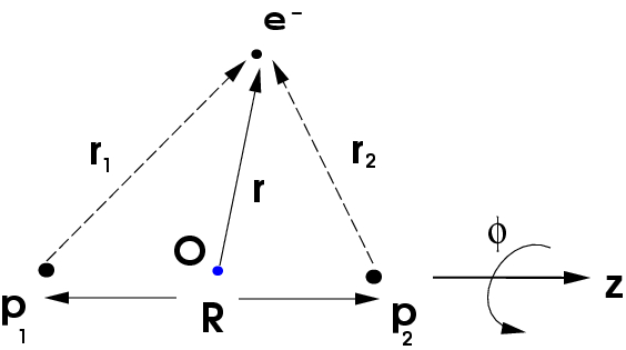
The origin, which lies midway between the two protons on the \(z\) axis, is shown as the blue dot. The position vector of the electron is \(r\). Denoting the positions of the two protons \(P_1\) and \(p_2\) as \(R_1\) and \(R_2\), respectively, we see that these vectors are simply:
\[R_1=\left(0,0,-{R \over 2}\right)\]
\[R_2=\left(0,0,{R \over 2}\right)\]
since the line joining the two protons is assumed to lie along the \(z\)-axis. The Hamiltonian for the \(H_2^+\) molecule ion, assuming the two protons are fixed in space, is
\[H= -{\hbar^2 \over 2m}\nabla^2 - {e^2 \over \vert{\bf r}-{\bf R}_1\vert} -{e^2 \over \vert{\bf r}-{\bf R}_2\vert} + {e^2 \over R}\]
=
Also, using the vectors \(r_1\) and \(r_2\) for the position of the electron with respect to the two protons, respectively, the Hamiltonian can be written in shorthand form as
\[H = -{\hbar^2 \over 2m}\nabla^2 - {e^2 \over r_1} - {e^2 \over r_2} + {e^2 \over R}\]
where it should be kept in mind that \(r_1\) and \(r_2\) are functions of \(r\), the coordinates of the electron with respect to our chosen coordinate system. Note that the term \(e^2/R\)is just a constant, representing the Coulomb repulsion between the two protons. We can, therefore, define the electronic Hamiltonian, \(H_{el}\) as
\[H = H_{\rm el} + {e^2 \over R}\]